One line code change → Save thousands

Benchmarking x86 vs ARM on GCP using a cheminformatics pipeline. One build flag reduced CPU costs by over 50%, with zero changes to application logic.

Aug 04, 2025

Large-scale molecular processing, like generating 3D structures from SMILES, is a core step in modern drug discovery pipelines. But when you're working with millions of compounds, even small inefficiencies can lead to significant cloud spend.

In this post, I’ll share how we benchmarked different CPU architectures on Google Cloud using a real-world cheminformatics pipeline, and how switching architectures with a single-line tweak in our container build process slashed our compute costs without modifying the application logic.

If your workloads are CPU-bound and containerized, this small optimization might translate into substantial savings at scale.

Context and Motivation

One of the most common steps in cheminformatics workflows is converting SMILES strings into three-dimensional molecular structures. While this step is relatively inexpensive at small scale, it becomes significantly more resource-intensive when applied to millions of compounds.

Because scientific workloads are not always optimized for a single CPU architecture, I wanted to compare four machine types available on Google Cloud (each with 4 vCPUs and similar hourly prices):

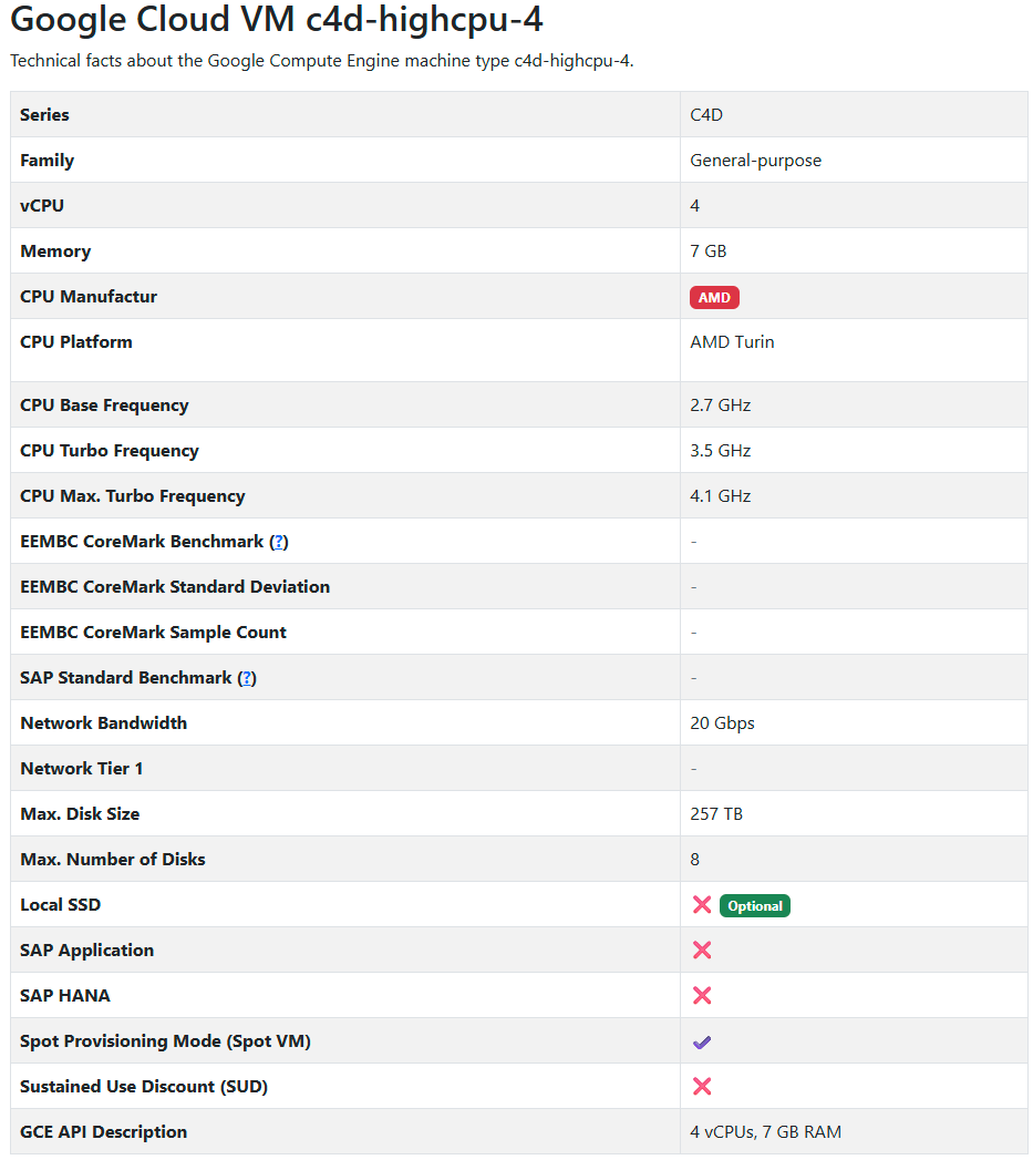
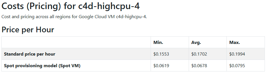
AMD (c4d-highcpu-4)
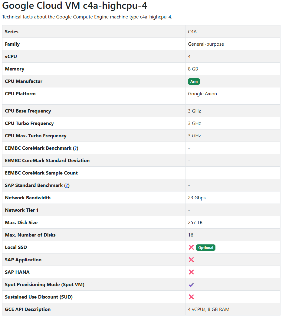
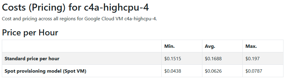
ARM (c4a-highcpu-4)
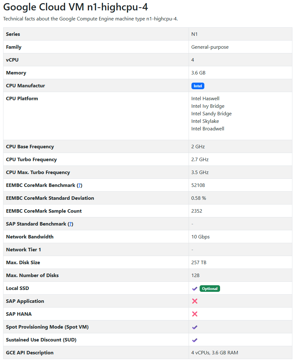
Intel N1 (n1-highcpu-4)
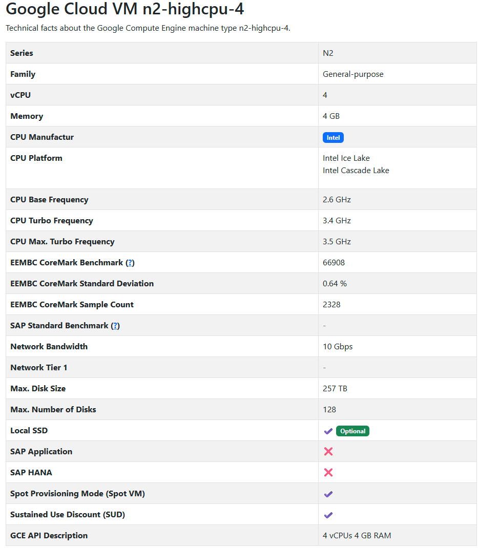
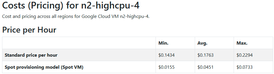
Intel N2 (n2-highcpu-4)

Note: All machines used had 4 vCPUs, but differed in CPU architecture, memory configuration, and performance characteristics.

For further details, see Appendix A (Machine Specs) and Appendix B (Pricing).

The goal was to determine which of these options offers the best performance per dollar, rather than focusing purely on execution speed.

Machine naming convention:

For simplicity and readability, the following shorthand will be used throughout this text to refer to the machine types:

AMD → c4d-highcpu-4

ARM → c4a-highcpu-4

INTEL_1 → n1-highcpu-4

INTEL_2 → n2-highcpu-4

Benchmark Design

We used a curated set of 1131 FDA-approved molecules from the Enamine catalog, representative of real-world pharmaceutical research scenarios. These molecules provide structural diversity and clinical relevance, making them an excellent test case for benchmarking performance.

The pipeline was run multiple times on each architecture under consistent conditions in the us-central1 region.* For each run, we measured:

Total execution time
Environment startup time
Estimated job cost, based on hourly pricing for each machine type

These raw measurements were then used to compute the key performance and cost-efficiency metrics presented in the next section, including per-molecule cost and overall throughput.

*This region was selected because it is one of Google Cloud’s most commonly used and broadly available zones, with wide support across all CPU architectures.

It also provides a balanced baseline in terms of latency, resource availability, and pricing consistency.

Choosing a general-purpose region like us-central1 helps ensure that the comparison reflects typical production conditions and is reproducible by other users.

Evaluation Metrics

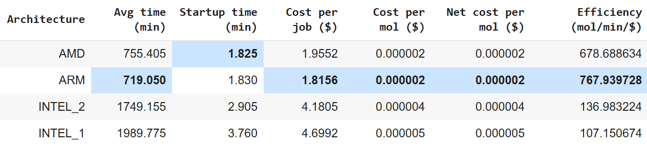
To evaluate performance and cost, I focused on six primary metrics:

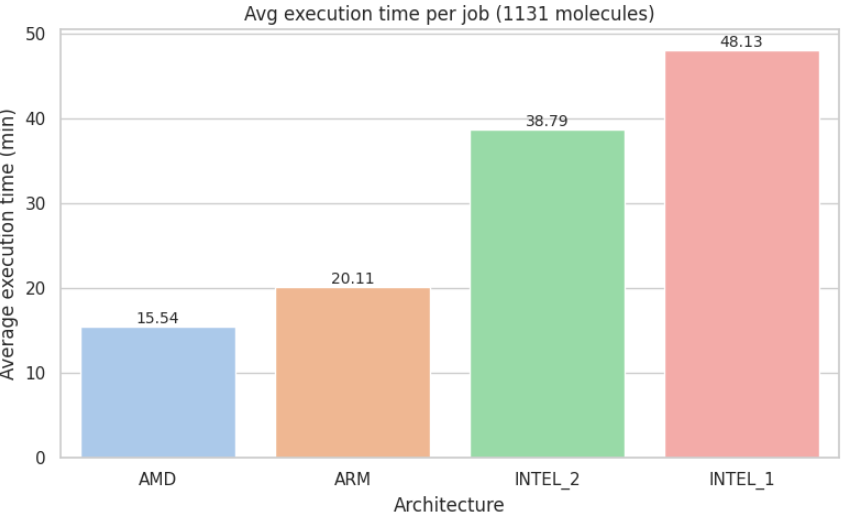
Average execution time per job (in minutes)

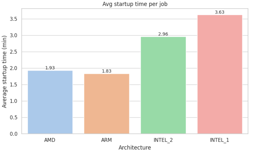
Average startup time (in minutes)

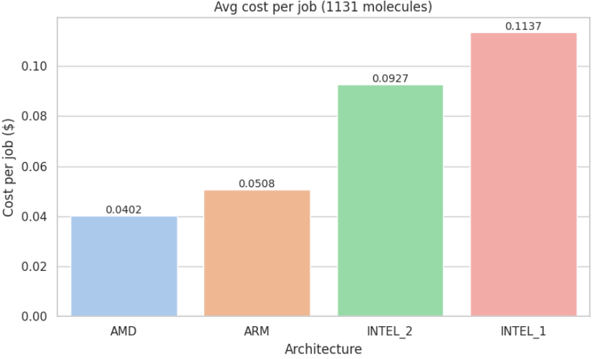
Average cost per job (in USD)

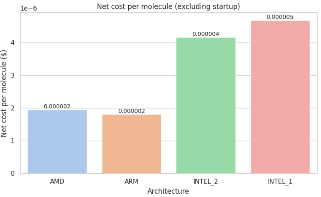
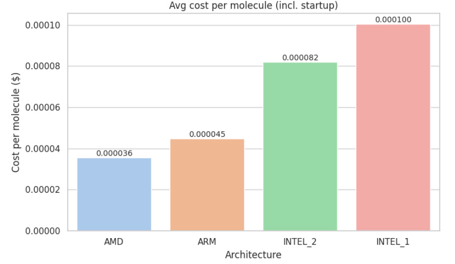
Average cost per molecule (in USD)

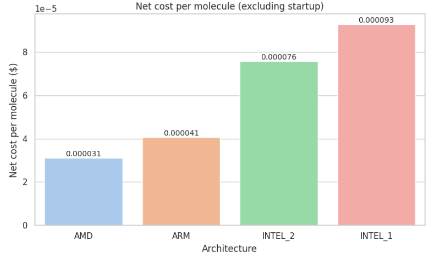
Net processing cost per molecule (in USD)

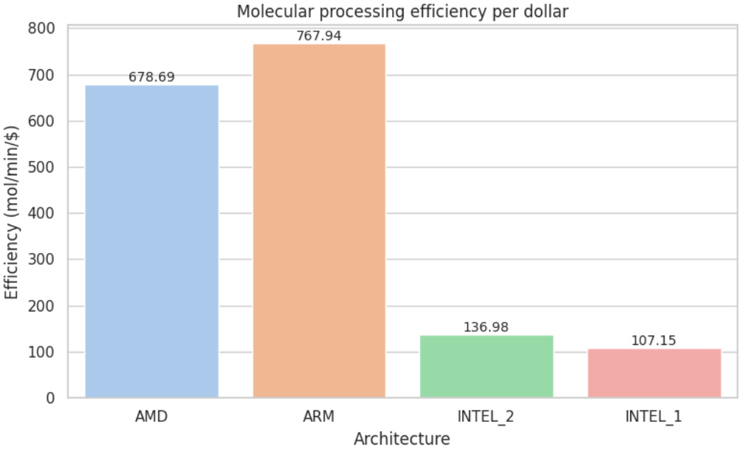
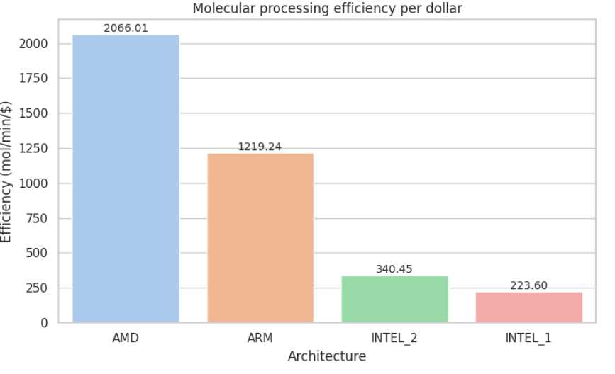
Efficiency (mol/min/$)

The net processing cost per molecule excludes the initial environment startup time from the total job duration. It is calculated as:

(Elapsed time − Startup time) × Price per hour / Number of molecules

This is particularly important because in real-world drug discovery workflows, pipelines often run for hours or even days, processing millions of molecules. In those scenarios, the fixed startup time becomes negligible. By removing that overhead, this metric provides a more realistic estimate of true compute efficiency per molecule, especially for high-throughput production settings.

The efficiency is defined as:

Efficiency = Molecules processed / (Net processing time × Cost)

This metric captures both speed and cost-efficiency, rewarding architectures that process the most molecules in the shortest time for the lowest total cost.

Rather than isolating speed or pricing alone, it helps identify the best return on investment (ROI) in compute resources, which is especially relevant in large-scale molecular pipelines, where cost per molecule and throughput per dollar are critical factors for controlling infrastructure spending.

Switching Architectures: Just a Few Lines of Code

One of the most surprising takeaways from this experiment is how minimal the effort was to switch architectures and reap the cost savings.

All it took was:

Updating the Dockerfile to target the new architecture (e.g., using --platform=linux/arm64 for ARM)

Rebuilding the container image

Redeploying the pipeline with the corresponding machine type (e.g., c4a-highcpu-4 for ARM)

There were no code changes required in the application logic. The underlying pipeline, including scientific libraries and dependencies, worked seamlessly across architectures thanks to multi-arch support in modern container toolchains.

If you're already using containers, this optimization could be just a one-line change in your build or deploy script, and worth thousands in compute savings at scale.

To take it a step further, we built a single multi-architecture Docker image using docker buildx, compatible with both ARM and x86 platforms.

This approach simplifies deployment, reduces architecture-specific bugs, and ensures portability across AMD, Intel, and ARM environments.

Bonus: How We Handle Multi-Architecture Builds

To make our pipeline portable across ARM and x86 machines, we configure our builds using Docker Buildx, and conditionally install architecture-specific binaries inside the container, such as the Micromamba distribution for linux-aarch64 or linux-64.

We also use ARG TARGETARCH in the Dockerfile to detect the build architecture and fetch the right version of tools like Micromamba. This allows us to install Open Babel and other dependencies reliably regardless of CPU type.

In our Google Cloud Build config, we dynamically install Buildx (if needed), create a builder, and then push a multi-platform image that works across all CPU types:

```yaml

--platform=linux/amd64,linux/arm64

```

Combined with a conditional logic block in the Dockerfile:

```dockerfile

ARG TARGETARCH

...

if [ "$TARGETARCH" = "arm64" ]; then ARCH=linux-aarch64; else ARCH=linux-64; fi

```

we ensure full compatibility without maintaining separate Dockerfiles for each architecture.

This approach keeps builds deterministic, avoids surprises, and allows any team member to deploy or test on any platform, without special configuration.

From Metrics to Results

With all evaluation criteria clearly defined, we applied them to benchmark the performance of the four selected architectures. Each job processed the same 1,131 FDA-approved molecules, and the pipeline was executed under consistent configuration and region settings.

The aggregated results per architecture are shown below, providing a comprehensive overview of how each machine type performed in terms of time, cost, and overall efficiency.

For visual comparison, see Appendix C: Metric Visualizations

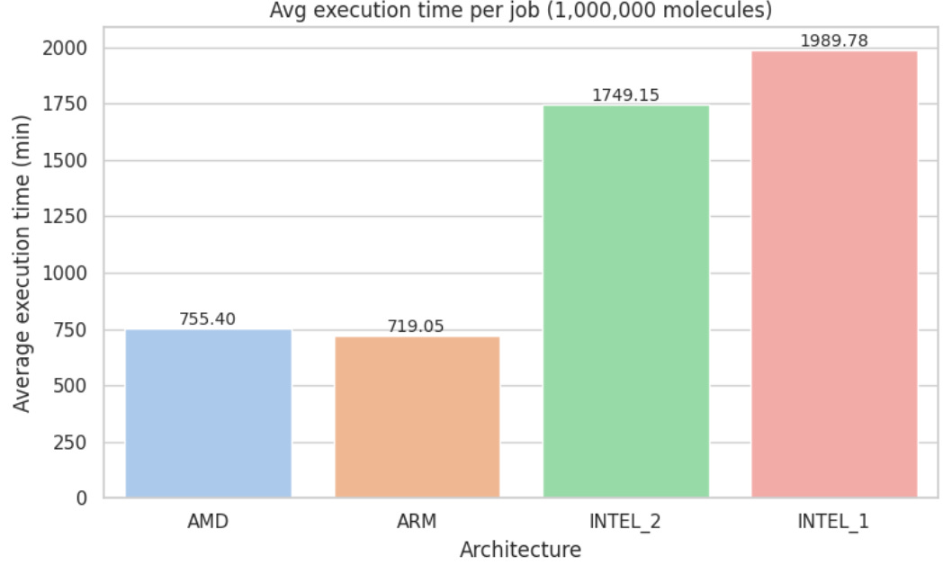
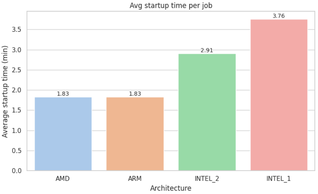
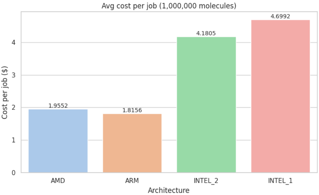
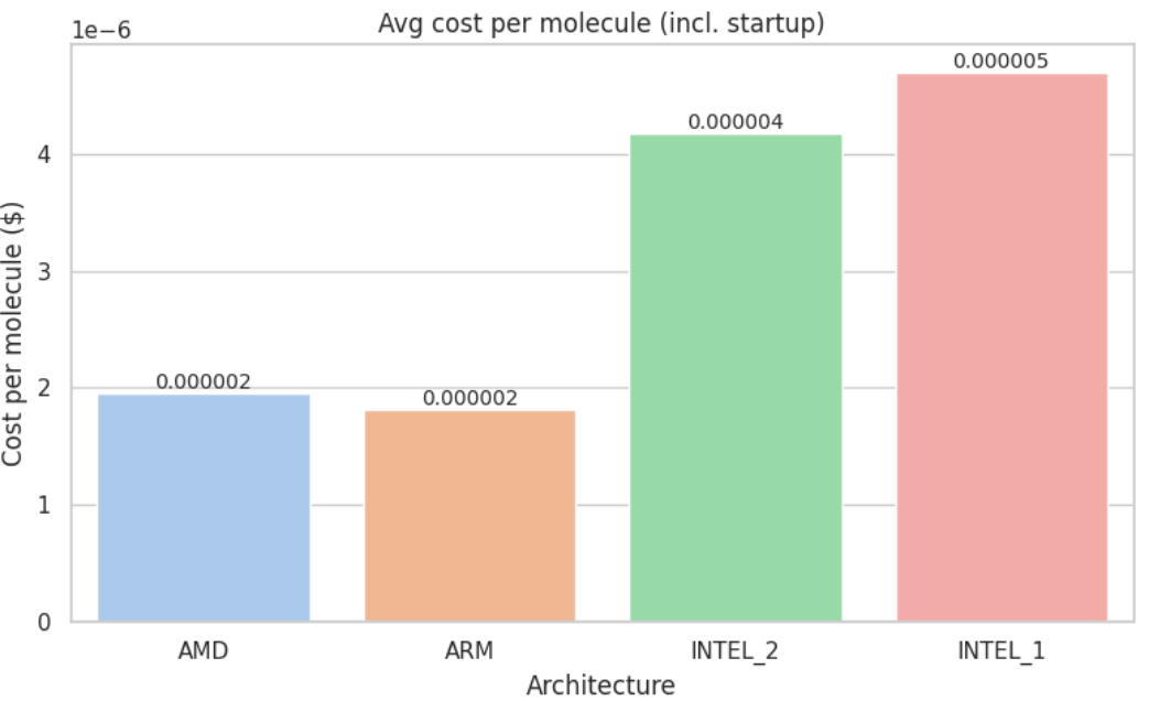
Large-Scale Benchmark: One Million Molecules

While the 1,131-molecule benchmark is useful for quick comparisons, real-world drug discovery workloads often involve millions of compounds.

To test how our findings hold at production scale, we repeated the same benchmark with 1,000,000 ligands, under identical conditions and pipeline logic.

For visual comparison, see Appendix D: Metric Visualizations

Conclusion

Across all metrics evaluated, the picture now depends on scale:

Small-scale benchmark (1 131 molecules).

The AMD (c4d-highcpu-4) instance once again outperformed the alternatives, offering the best balance of execution speed, cost-efficiency, and overall molecular throughput. ARM (c4a-highcpu-4) followed closely in cost-effectiveness, making it a viable secondary option.

Large-scale benchmark (1 000 000 molecules).

When we pushed the pipeline to production scale, ARM moved into first place: it completed the job about 5 % faster than AMD, drove the job cost down by roughly 7%, and delivered ~13 % more molecules-per-minute-per-dollar. AMD remained a very strong performer, but ARM now offers the best return at this workload.

In contrast, Intel-based instances (n1 and n2 families) continued to show substantially higher execution times and costs, resulting in markedly lower efficiency per dollar in both tests.

If your workloads are similar (CPU-bound, highly parallelizable, and run at the million-ligand scale) I recommend testing ARM-based instances first. For smaller batches or situations where x86-64 compatibility is critical, AMD remains an excellent choice.

These findings demonstrate the value of benchmarking real workloads across architectures and at the right scale. Small differences in pricing and speed can scale into significant cloud-cost savings (or overruns) when a pipeline moves to production.

Thanks for reading Pauling AI Blog! This post is public so feel free to share it.